Computer Aided Geometric Design
Bezier Curves

Introduction
The de Casteljau Algorithm
Geometric Continuity

Introduction

Engineers of the automotive industry created the first geometric models in the 1960’s,and so initiated the domain of CAGD. Beginning in the 1960’s, engineers designing carbody parts started to use computers, an emerging technology, to represent the surfaces they were to produce. Parametric surfaces which had been long known and studied by mathematicians are well suited for representing these surfaces. Nevertheless ﬁnding appropriate numerical representations for these surfaces and tools adapted to manipulate them was a completely new task, and therefore developing these new representations was the ﬁrst goal of the pioneers of the field. These new representations for surfaces, using intuitive numeric parameters to control their shape, quickly made their way to other manufacturers: from car bodies, to airplanes, to mechanical parts. The need for geometric modeling rapidly extended to other domains–to medicine, to architecture, and to geology– following the growing inﬂuence of computers. More recently, virtual worlds have also used geometric models, for the conception of physical shapes or simply for representing non physical objects. With the role of computers always increasing,the need for geometric models is growing too. The increase in computational power allows richer models to be developed, and users expect the manipulation tools and algorithms to be increasingly efficient and to offer more and more functionality. The ability to understand, construct and process three-dimensional geometric models on the computer is essential for many modern engineering fields, such as computer-aided design and manufacturing (CAD/CAM), engineering simulation, biomedical imaging, robotics, computer vision, and computer graphics. We focus here on CAGD techniques for modeling freeform curves and surfaces such as body shapes of ships, automobiles and aircrafts. Many consumer products as well as electronic devices are also designed with freeform aesthetic shapes. For this, we need to define the concept of Bezier Curves. Pierre Bezier was a French Arts & Métiers engineer (Pa27) who did his career at Renault.

Linear Bezier curve

Linear Bezier parametric curve is obtained by linear interpolation between two given control points $P_{0}$ and $P_{1}$ in the plane.

For all 0 \leq t \leq 1, BP [P_{0}, P_{1}] (t) = (1 - t) P_{0} + t P_{1}

Use your finger or mouse to move nearest control point (the small blue circles)

Here, $BP$ , means Bezier Polynomial parametric curve. In the right window, you can see the basis polynomials of the linear Bezier curve. The red line is $(1 - t)$ and the green one is $t$ . In this example, the list of control points is $P$ =[[0.1,0.1],[0.9,0.9]]

More generally, we have the following definition of Bezier curves:

Let us given

n + 1

points

P_{0}, . . ., P_{1}

, we call Bezier curve a polynomial parametric curve defined by:

For all 0 \leq t \leq 1, BP [P_{0}, P_{1}, . . ., P_{n}] (t) = B_{0}^{n} (t) P_{0} + B_{1}^{n} (t) P_{1} + . . . + B_{n}^{n} (t) P_{n}

where the

B_{i}^{n} (t) = C_{n}^{i} (1 - t)^{n - i} t^{i}

for

i = 0, . . ., n

are the Bernstein polynomials of order

n

with

C_{n}^{i} = \frac{n!}{i! (n - i)!}

Quadratic Bezier curve

Quadratic Bezier curve is obtained from three control points $P_{0}$ , $P_{1}$ and $P_{2}$ . The Bezier curve is then defined by: $For all 0 \leq t \leq 1, BP [P_{0}, P_{1}, P_{2}] (t) = B_{0}^{2} (t) P_{0} + B_{1}^{2} (t) P_{1} + B_{2}^{2} (t) P_{2}$ where the $B_{0}^{2} (t) = (1 - t)^{2}$ , $B_{1}^{2} (t) = 2 t (1 - t)$ and $B_{2}^{2} (t) = t^{2}$ are the Bernstein polynomials of order $2$ . They define a basis of the vector space of polynomials of degree less or equal to $2$ . To the right you can see basis polynomials $B_{0}^{2} (t)$ , $B_{1}^{2} (t)$ and $B_{2}^{2} (t)$ in the red, green and blue order.

By construction Bezier curve goes through its terminal control points ( $P_{0}$ and $P_{2}$ here) and is tangent to the first and last segments of the control polygon. As we can, the Bezier curve "mimics" the shape of the control polygon. This can be possible due to the properties of the Bernstein polynomials. Usually, it is very difficult to design a polynomial curve when the curve is written in the canonical basis. This change of basis creates good visual conditions for "easy" design of the curves.

Cubic Bezier curve

In a similar way, for

n = 3

, we get a cubic Bezier curve

Bezier curve of degree $n = 7$

The initial control points are given by the following list:

P

= [[0.1,0.1],[0.1,0.8],[0.8,0.9],[0.8,0.2],[0.5,0.1],[0.3,0.5],[0.5,0.6],[0.9,0.3]]

On the right, we can see all the Bernstein polynomials

B_{i}^{n} (t)

for

i = 0, . ., 7

needed to design this Bezier parametric curve.

By moving the control points (blue circles), you can see that the red curve, is always located in the convex hull of the control points of the Bezier curve. This property can be demonstrated.

The de Casteljau Algorithm

In 1958, Paul Faget de Casteljau engineer at Citroën, developped a simple algorithm which allows to calculate the value of $BP (t)$ for any given value of $t$ .
For example if $n = 2$ then his algorithm is defined as follows. We fix the value of $t$ (for example $t = \frac{1}{2}$ ) and we calcute the two points $P_{0}^{(1)}$ and $P_{1}^{(1)}$ respectively the middle points of segments $[P_{0}, P_{1}]$ and $[P_{1}, P_{2}]$ .
They are calculated as follows for $t = \frac{1}{2}$ : $\begin{array}{l} P_{0}^{(1)} = (1 - t) P_{0} + t P_{1} \\ P_{1}^{(1)} = (1 - t) P_{1} + t P_{2} \end{array}$ Finally, by iterating again this barycentric calcultation we obtain: $P_{0}^{(2)} = BP (t) = (1 - t) P_{0}^{(1)} + t P_{1}^{(1)}$ Note that $P_{0}^{(2)}$ subdivides the Bezier curve in two quadratic curves. The new curves match the original in position, although they differ in parameterization. The two polygons $[P_{0}, P_{0}^{(1)}, P_{0}^{(2)}]$ and $[P_{0}^{(2)}, P_{1}^{(1)}, P_{2}]$ are the control polygons of two new bezier curves that match perfectly the initial one.

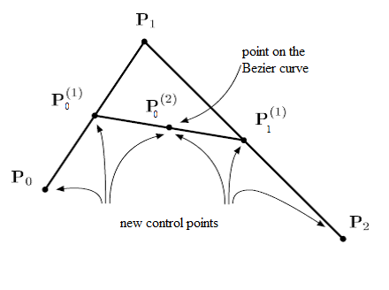
In the following Figure, the two points $P_{0}^{(1)}$ and $P_{1}^{(1)}$ are the extremeties of the green segment and the point $P_{0}^{(2)}$ is the black point. They are calculated by the de Casteljau algorithm for different values of $t = \frac{i}{100}$ for $i = 0, . ., 100$ . Consequently, by joining all these black points it is possible to draw the Bezier curve in red. We then don't need to calculate the Bernstein polynoms.

More generally, Paul de Casteljau demonstrated the following theorem:

Let us given

n + 1

points

P_{0}, . . ., P_{n}

and

j

be a fixed integer of {0,...,n}. It yields:

For all 0 \leq t \leq 1, BP (t) = B_{0}^{n - j} (t) P_{0}^{(j)} + B_{1}^{n - j} (t) P_{1}^{(j)} + . . . + B_{n}^{n - j} (t) P_{n - j}^{(j)}

where

P_{i}^{(0)} = P_{i}

and

P_{i}^{(j)} = (1 - t) P_{i}^{(j - 1)} + t P_{i + 1}^{(j - 1)}

for

i = 0, . . ., n - j

Exercice[de Casteljau Algorithm]

We want to draw a Bezier curve by using the de Casteljau algorithm.

Plot all the Bernstein polynomials for $n = 3$ . For this, use the following binomial function.

                    
    import numpy as np
    from math import factorial as fac
    
    def binomial(n,i):
        try:   
            binom=fac(n)/(fac(i)*fac(n-i))
        except ValueError:
            binom=0.0              
        return binom

    def bernstein(n,i,t):
        #TO DO               
        return 

            
        

        def bernstein(n,i,t):
            res=binomial(n,i)*(1-t)**(n-i)*t**i
            return res

        t=np.linspace(0,1,100)

        n=3
        for i in range(n+1):
            y=[bernstein(n,i,x) for x in t]
            plt.plot(t,y)
        plt.show()

By using the result of the previous Theorem, implement the de Casteljau function for $j = n$ . This function will return the value of $BP (t)$ for a given $t$ . $P$ is the list of the control points of the Bezier curve.

                    
    import numpy as np

    def decast(t,P):
        #TO DO    
        return

        def decast(t,P):
            n=len(P)-1
            L0=P
            for k in range(n):
                L=L0
                L0=[]
                for i in range(n-k):
                    L0.append(np.dot(1-t,L[i])+np.dot(t,L[i+1]))
            return L0[0][0],L0[0][1]

By using the previous decast function, draw the cubic Bezier curve with control polygon $P = [[0.1, 0.1], [0.9, 0.9], [0.1, 0.9], [0.9, 0.1]]$ . For this you can use a subdivision of $[0, 1]$ by using np.linspace(0,1,100). Calculate for each values the corresponding values of the Bezier curve. The drawing of the Bezier curve is obtained by joining all these values. As in the previous Bezier examples you can draw also this control polygon.

                    
    import numpy as np
    import matplotlib.pyplot as plt

    def DrawBezier(P,nb=100):
        #TO DO    
        return

        def DrawBezier(P,nb=100):
            z=np.linspace(0,1,nb)
            X=[]
            Y=[]
            for t in z:
                x,y=decast(t,P)
                X.append(x)
                Y.append(y)
            return X,Y
    
        P=[[0.1,0.1],[0.9,0.9],[0.1,0.9],[0.9,0.1]]
        p=np.transpose(P)
        X,Y=DrawBezier(P)
        # Plot the control polygon of the Bezier curve
        plt.plot(p[0],p[1],'r')
        plt.plot(X,Y)
        plt.show()

Geometric Continuity

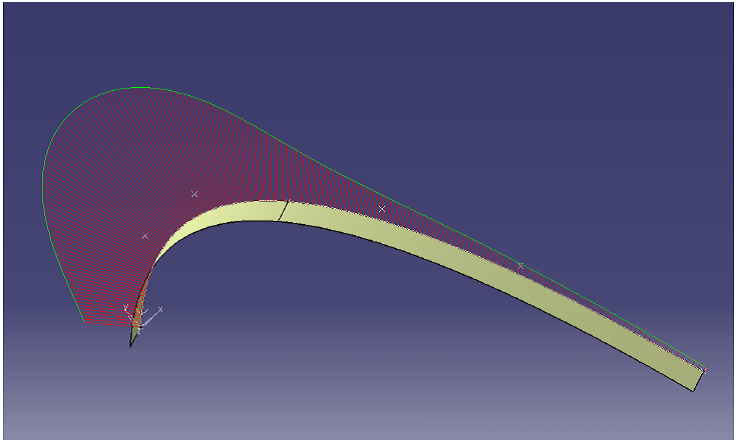
In practice, the modeled objects can be produced from several Bézier curves. In the following example, the two curves are joined with the $C^{3}$ continuity. This was done with CATIA V5.

To guarantee a certain regularity of fitting, it is necessary to know how to calculate the derivatives of a Bézier curve. The following proposition makes it possible.

Let us give

n + 1

data points

P_{0}, \dots, P_{n}

R^{d}

(

d = 2, 3, . . .

) then the derivative of order

k \in I N

is given by

\forall t \in [0, 1], \frac{d^{k} BP [P_{0}, P_{1}, \dots, P_{n}]}{d t^{k}} (t) = \frac{n!}{(n - k)!} \sum_{i = 0}^{n - k} B_{i}^{n - k} (t) Δ^{k} P_{i},

where

Δ^{k} P_{i}

is the operator of progressive differences of order

k

at point

P_{i}

For example we have:

Δ^{1} P_{i} = P_{i + 1} - P_{i} = \vec{P_{i} P_{i + 1}}

Δ^{2} P_{i} = Δ^{1} (Δ^{1} P_{i}) = P_{i + 2} - P_{i + 1} - P_{i + 1} + P_{i} = \vec{P_{i + 1} P_{i}} + \vec{P_{i + 1} P_{i + 2}}

.
Moreover,

Δ^{k} P_{i} = Δ^{1} (Δ^{k - 1} P_{i}) = \sum_{j = 0}^{k} (\binom{k}{j}) {(- 1)}^{k - j} P_{i + j}

.
Consequently, we have at the extremities:

\frac{d^{k} BP [P_{0}, P_{1}, \dots, P_{n}]}{d t^{k}} (0) = \frac{n!}{(n - k)!} Δ^{k} P_{0}

\frac{d^{k} BP [P_{0}, P_{1}, \dots, P_{n}]}{d t^{k}} (1) = \frac{n!}{(n - k)!} Δ^{k} P_{n - k}

Exercice [ $C^{3}$ -continuity]

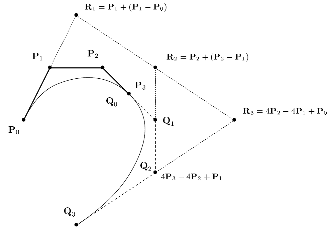
In this exercice, we wish to build a cubic Bezier curve with unknow control polygon $Q = [Q_{0}, Q_{1}, Q_{2}, Q_{3}]$ which joined $C^{3}$ -continuously with a given Bezier curve (See the following Figure)

Let us give the cubic Bezier curve with control polygon $P = [P_{0} = [0.1, 0.1], P_{1} = [0.9, 0.9], P_{2} = [0.1, 0.9], P_{3} = [0.9, 0.1]]$ , by using the previous proposition calculate the $C^{0}$ , $C^{1}$ , $C^{2}$ and $C^{3}$ derivatives at $t = 0$ and $t = 1$ respectively.
By using the previous results, calculate the values of points $Q_{0}$ , $Q_{1}$ , $Q_{2}$ and $Q_{3}$ such that this cubic Bezier curve joins $C^{3}$ at $t = 0$ with the cubic Bezier Curve with control polygon $P$ at $t = 1$ .
Draw these two Bezier curves.

C^{0} :

BP [Q] (0) = BP [P] (1)

Consequently

Q_{0} = P_{3}

C^{1} :

\frac{d BP [Q]}{d t} (0) = \frac{d BP [P]}{d t} (1)

Consequently

Q_{1} - Q_{0} = P_{3} - P_{2}

, it yields that

Q_{1} = P_{3} + (P_{3} - P_{2})

C^{2} :

\frac{d^{2} BP [Q]}{d t^{2}} (0) = \frac{d^{2} BP [P]}{d t^{2}} (1)

Consequently

Q_{2} - 2 Q_{1} + Q_{0} = P_{1} - 2 P_{2} + P_{3}

, it yields that

Q_{2} = P_{1} + 4 (P_{3} - P_{2})

C^{3} :

\frac{d^{3} BP [Q]}{d t^{3}} (0) = \frac{d^{3} BP [P]}{d t^{3}} (1)

Consequently

Δ^{3} Q_{0} = Δ^{3} P_{0}

, it yields that

Q_{3} = . .

        P=[[0.1,0.1],[0.9,0.9],[0.1,0.9],[0.9,0.1]]
        p=np.transpose(P)
        X,Y=DrawBezier(P)
        # Plot the control polygon of the Bezier curve
        plt.plot(p[0],p[1],'r')
        plt.plot(X,Y)

        # Calculate the control polygon Q for the C2-continuity 
        Q0=P[2]
        Q1=Q0+(np.add(P[2],np.dot(-1,P[1])))
        Q2=np.add(P[0],np.dot(4,(np.add(P[2],np.dot(-1,P[1])))))
        # in this case Q3 is free of constraint
        Q3 = [1,1]
        Q=[Q0,Q1,Q2,Q3]
        q=np.transpose(Q)
        X,Y=DrawBezier(Q)
        plt.plot(q[0],q[1],'r')
        plt.plot(X,Y)

        plt.show()

        # for the C3 case, the location of Q3 is given by defining
        # the symmetric point of R3 (see the previous Figure)
        # You can calculate it by ourself.

References

J.H. Ahlberg, E.N. Nilson & J.L. Walsh (1967) The Theory of Splines and Their Applications. Academic Press, New York.
C. de Boor (1978) A Practical Guide to Splines. Springer-Verlag.
G.D. Knott (2000) Interpolating Cubic Splines. Birkhäuser.
H.J. Nussbaumer (1981) Fast Fourier Transform and Convolution Algorithms. Springer-Verlag.
H. Späth (1995) One Dimensional Spline Interpolation. AK Peters.

Computer Aided Geometric Design Bezier Curves

Introduction

The de Casteljau Algorithm

Exercice[de Casteljau Algorithm]

Geometric Continuity

Exercice [C3-continuity]

References

Computer Aided Geometric Design
Bezier Curves

Exercice [ $C^{3}$ -continuity]